I worked on interval aithmetic using numpy this week. I have almost got the module ready. I have to integrate it with Stefan’s branch and a basic version of implicit plotting will be ready to go. I will update this blog post with plots and performance results once I integrate it with Stefan’s branch.
Adaptive Sampling for 2D Plots
This was my first week of GSoC and I spent time on experimenting with adaptive sampling. The major idea explored were what constitutes a condition for which we need not sample more to obtain an accurate plot. I started with the idea of the area of the triangle formed by the three consecutive points to be less than a tolerance value. This worked nicely but did oversampling unnecessarily. The problem with it was the area of the triangle was dependent on the distance between the points which made the condition dependent on the lengths and hence oversampled even though the line formed by the three points was almost collinear. So the obvious next idea was to check the angle formed by the three points and see whether it forms an angle near to 180 degree. There were three versions of the above algorithm implemented, out of which one was the iterative version of a recursive solution. The iterative version is here. Considering Stefan Krastanov’s suggestion, I implemented a recursive solution which samples 5 additional points between two points instead of a single point. The idea was to use numpy’s quick evaluations of an array and also arrive at the straight line condition faster. Also, this reuses most of the code written before. The code for the following can be found here. The snippet of the code is as follows:
1 2 3 4 5 6 7 8 9 10 11 12 13 14 15 16 17 18 19 20 21 22 23 24 25 26 27 28 29 30 31 32 33 34 35 36 37 | |
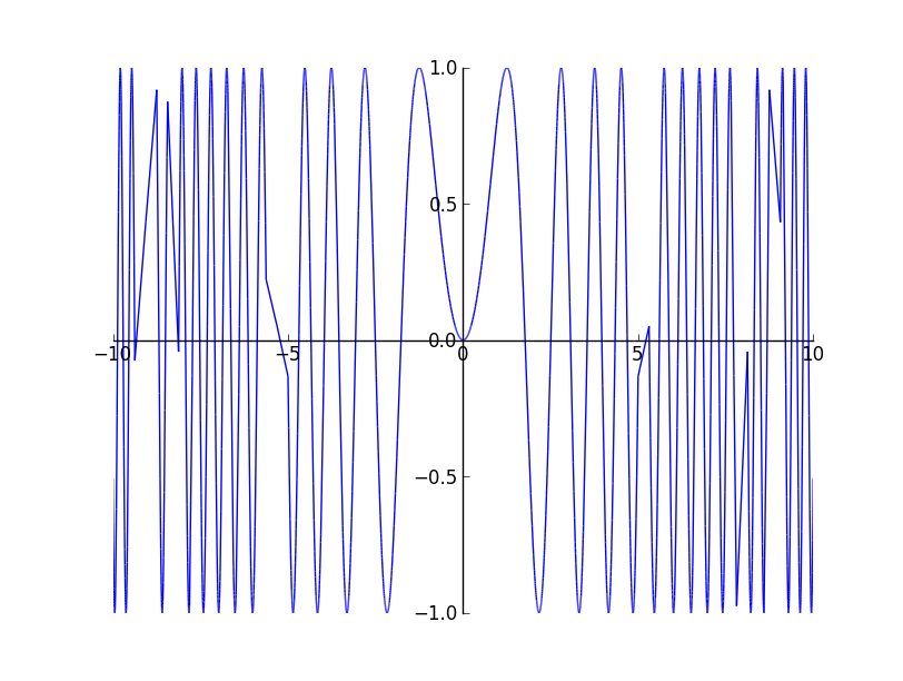
The major problem with the above approach is the way that the rightmost point / segment is handled. The rightmost segment does not have another right segment to decide whether it forms a 180 degree angle or not. Hence it is assumed straight if the previous segment and the present segment forms a straight line. Most of the time this fails to sample further for the end segment thought it should have sampled. The problem can be seen in an plot of $y = sin(x^{2})$
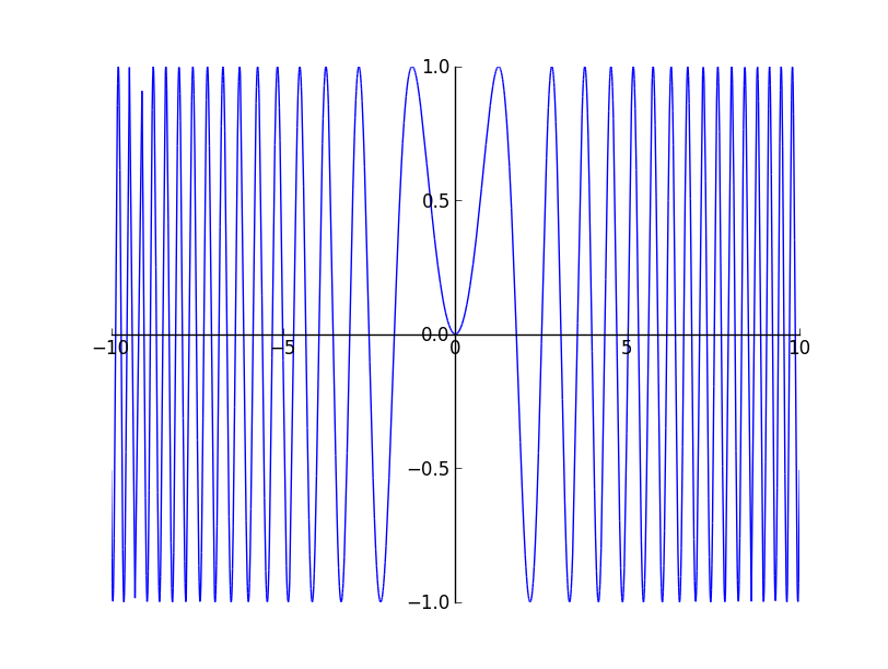
The last method used is symmetric and gives better results, but it is quite ugly. The branch is here.(EDIT: changed the link). It uses some amount of random sampling to avoid aliased results. The plot of $y = sin(x^{2})$ renders very accurately. Feel free to experiment with it and if there is a better method, you can comment below :).
I think I will get an non - ugly code ready by the tomorrow and wait for Stefan’s branch to get merged before submitting this method as pull request. This week has been lots of experimentation. I think I will spend the next week getting a basic version of Interval Arithmetic ready using numpy.
Region Plots With Interval Arithmetic
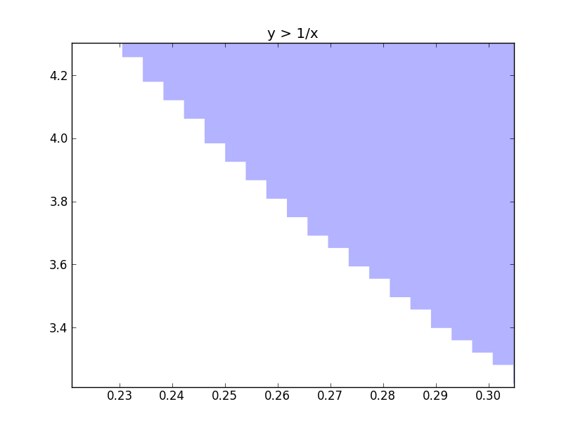
My GSoC project is to provide support for implicit plotting using interval arithmetic. As mpmath already has a very good interval arithmetic library, I wanted to try out how efficient the algorithm is going to be using the mpmath interval arithmetic library. I wanted to get an idea on the time required for plotting and also wanted to decide whether to write my own interval arithmetic library or use the existing mpmath library and add additional things to it. I have a basic implementation which supports only the mpmath interval arithmetic functions. The results look promising and I am guessing a separate implementation for plotting will be faster and I will be able to add features more easily.I have an image of $y > 1/x$ with the interval edges below. The image below was plotted so with a resolution of 1024x1024. It is possible to see how the intervals are subdivided more and more when it reaches the edge of a region.
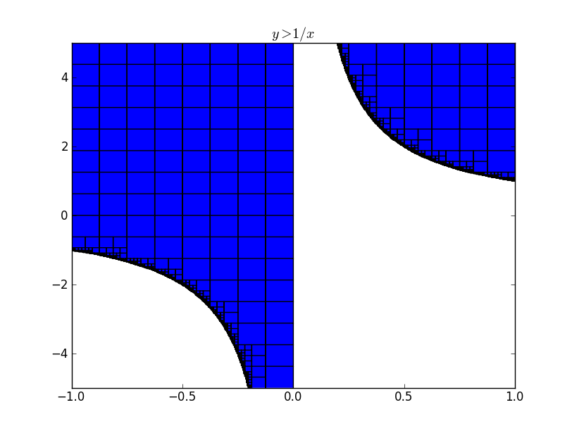
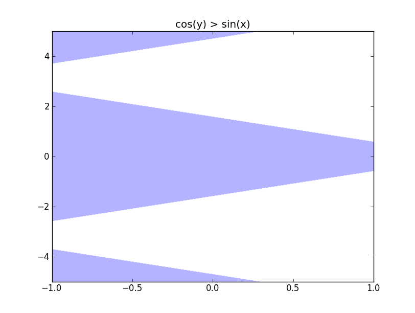
It took 1.57 seconds to render this image which is decently fast. I observed that if the independent regions are less and large, then the time take for the plot to be rendered is high. I tried $cos(y) > sin(x)$ which took about 5.3 seconds to render.
I wanted to try what the maximum time it takes to render something. So I tried plotting $sin^{2}x+cos^{2}x$ less than 1. As the arithmetic is done on intervals, it is not possible for the algorithm to decide that the expression is not true throughout the interval. So it goes on subdividing more and more, until it reaches a dimension of 1 pixel. For a resolution of 512X512, it took 120 seconds to render. If there are a lot of evaluations in the expression, then it might increase, but we should be expecting times around 120 seconds.
Another problem that I have to address is rasterization. I am really not getting any ideas on how to avoid rasterization. One way is to handle the zoom event in matplotlib and change the data to match the zoom. But for complicated graphs, revaluating might take a lot of time, which is bad.
We can see that if there is a way of interpolating over the rectangular edges, then we will have a plot without rasterization. I haven’t got any foolproof idea to implement this interpolation as there will be many independent regions. So if you have any idea, then please comment or mail me :). The code for plotting can be found here.
GSoC 2012 Sympy
I was selected by SymPy to work on their plotting module as part of GSoC2012. So I will be spending the next three months working on a plotting module to plot implicit functions. Implicit functions are difficult to plot by simple meshing. Though we might get a good result with simple meshing for most of the functions, it can be quite erroneous for some of the functions. So I will be using interval arithmetic to provide a way to plot implicit functions. My GSoC application can be found here. I will be atlast making a lasting contribution to an open - source software.
There are a lot of posts on how contributing to a open source software is the best way to sharpen your programming skills. But lot of people are too afraid to approach an organization and start contributing. There is an impending fear that people working on these projects are very stud(intelligent) people and they might get annoyed at your ignorance. Well, let me tell you this, people in an open source project are really nice. They don’t get annoyed very easily and they are ready to help you with everything. They correct all your mistakes with lots of patience and help you with improving your code. I think getting your code reviewed is the best way to improve your programming skills after you have reached a certain stage.
I was pretty much amazed with SymPy’s code base. Its so neat and clean that any newcomer can just look at the docstrings and can deduce the functionality of every function. Though my experience is limited, I haven’t seen a better codebase than SymPy’s. I am still looking at their codebase and the amount of modularity continues to amaze me. So if anybody is interested in contributing to a python open source project, then consider contributing to SymPy, for you will learn a lot on how a python project has to be structured.
I will be using this blog to update about my GSoC project and hopefully I will learn a lot during this period.
Hello World
Hello World
Its been a long time procrastinating to write a blog. Having read this post, I realized that I really need to think about the progress I am doing each day. I will be creating a new post every two days, in the worst case, with something that I have learnt or something that I know. Writing about something you know, really questions your assumptions, and you realize that you really didn’t know something that well. Its also been a long time that I wrote essays, and I am feeling rusty. It is reflected in the way that I am writing this post. It is high time that I improve my writing skills also. Hopefully I will imprve over time
I put a lot of effort to get this blog running. I feel really powerful as I can configure this blog as I want it to be and more than anything, it has MathJax support. I think this will help me to express my views better.