Bharath Mankalale

Gsoc Week 9

This has been a really unproductive week. I was sick with fever for almost three days and could not spend my time on anything. I spent the next days getting the basic svgfig backend for 2d line plots. There are lots of issues with svgfig, and hence I am of the opinion svgfig should be used only for displaying images on the google app engine ie sympy live. First on the list is no support for 3-D graphs. I think this is ok, because there are not many libraries even in javascript which can do 3D plotting. Also, I am having problems with implementing contour plots and surface plots in svgfig. I am experimenting with a way, which would involve using marching squares algorithm to plot contour plots.

I think I am a little behind my gsoc schedule, and I should speed up things a little in the next few weeks.

So these are the things that I have to address

  • Integration of svgfig with sympy live
  • Fix the multiple spawning of windows in matplotlib issue.
  • Fix the plot tests. As of now, the tests do nothing, as the process_series is not called if show is set to False.
  • I have been toying around with ipython to get isympy notebook and qtconsole working. The problem I am facing is, there are 2 instances of qtconsole created, instead of one, when I run it. I will have to figure out the problem.
  • Address the issues regarding the adaptive sampling of 2d plots.
  • Clean up my branch of implicit plotting (This is almost done).
  • Split the plot function into plot, plot3d, implicit_plot functions.

I don’t think I will be able to do all of these by the end of gsoc period. But my priority will be getting the implicit plotting and svgfig backend working and getting my pull requests merged.

GSoC Week 7

This week has been quite eventful. The implicit plotting module is almost done. I added the functionality of combining expressions using the And and Or statements. Now you can do

1
plot_implicit(And(Eq(y, exp(x)), y - x > 2)

and get a plot as below. So now you can combine any number of equations / inequalities and plot it. I think its possible to do a lot of cool stuff combining equations / inequalities.

Plotting through interval math is awesome but is also very limited. You cannot add support to re(), to functions that you cannot characterize as monotonic in certain regions. But we always encounter such functions. So there should be some fall back algorithm to plot such plots. I implemented the fall back algorithm last week. The idea is borrowed from sage implicit plots. We convert an equation / inequality into a function which returns 1 if it satisfies and -1 if it doesn’t satisfy. So if you are plotting an equality then you plot using the contour command of matplotlib, and instruct it to plot only the zero contour. If its an inequality then plotting the region with two colors gives the plot required.

These are examples from the fallback algorithm.

Plot of $y^{2}=x^{3}-x$

The plot with interval arithmetic is more precise.

I haven’t finished with the tests. Once I finish the tests I can send a pull request. The pull request will be pretty big, but most of the things have been reviewed in my previous pull request. This is just an extension of the previous pull request.

There are certain problems with the module though. The line width problem which I mentioned in my previous blog post, cannot be fixed. So you will have to change to the fall back method if the line width becomes large. Also the fall back algorithm cannot plot boolean combinations of equations / inequalities. So the two methods complement each other largely. So the next question would be whether we can choose one of the two intelligently. I guess the answer is No. That decision must be taken by the user. But most of the times the interval math approach works very nicely.

GSoC Week 6

I have been trying to improve the implicit plotting module during this week. But I have hit a road block. I almost ran out of ideas to solve the problem.

Description:

The implicit plotting algorithm I implemented works something like below:

1) Get x and y interval. If it satisfies the expression throughout the interval, then plot it.

2) If it does not satisfy, throw away the intervals.

3) If it partially satisfies, then recursively subdivide into four intervals, and try again.

For cases of equality, the first point never holds true due to floating point errors. So we go on eliminating regions, and after a certain depth, plot the remaining region. These are the regions where there is at least one solution. This is the reason why the plots are rasterized. But there is an inherent bigger problem here. In the cases of expressions like $x^{3}$ even if the x interval is small, the resulting interval after computation will be large. Sometimes, due to these large intervals, there might be lots of y and x intervals which satisfy because of these errors. Even if we make x interval really small, the corresponding y interval will be large, ie the line widths become large. The explanation is more of a guess rather than the right explanation.

Examples:

Plot of $x^{y}=y^{x}$ 
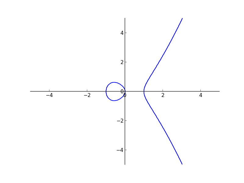
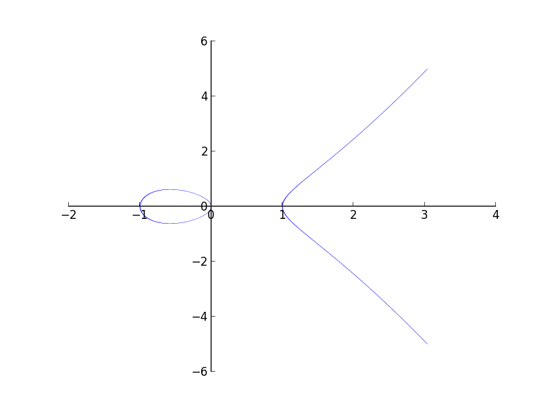
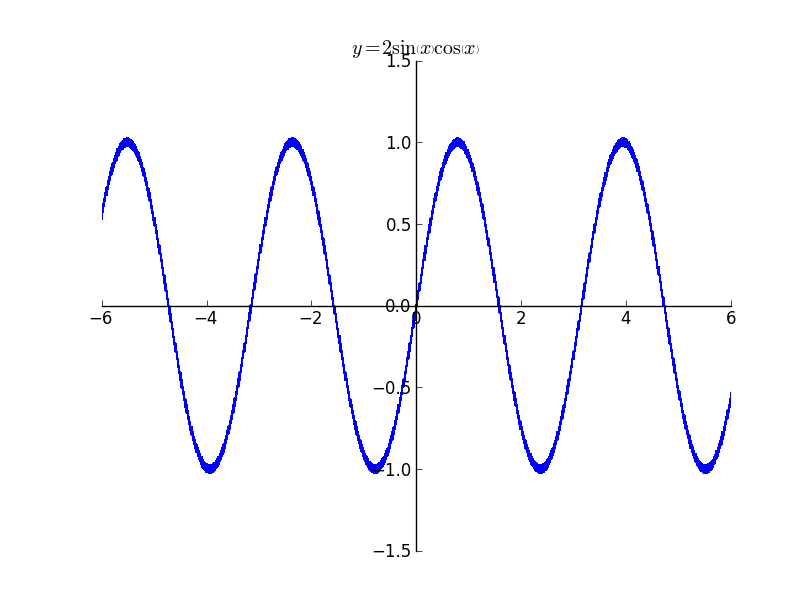
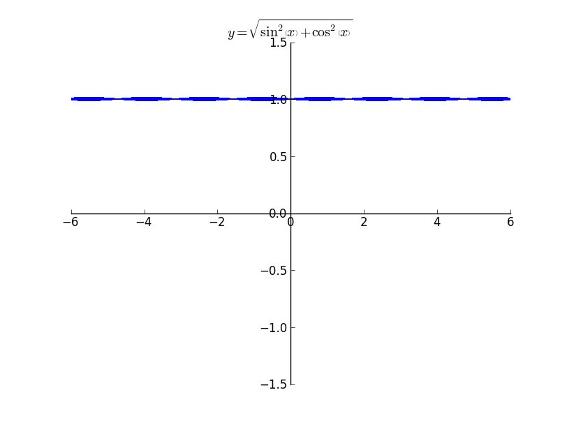
Even if I increase my depth of recursion to higher values, the thickness becomes less, but doesn’t vanish. The plot actually should have been two separate curves.

The Mac OSX’s Grapher uses a similar algorithm(A guess because they have similar rasterization) but takes care of the line widths.

If you feel you know where the problem is, please comment or email me. :)

Gsoc Week 5

This week has been mostly bug fixing and working on migrating the sympy ipython profile to sympy. I also wanted to add the functionality of ipython -c qtconsole. So it has been mostly hanging in the ipython irc, asking them lots of questions on how ipython works. I am really thankful to minrk who patiently taught me how to do most of the stuff. There are a few problems that I am facing, but I think I will have the qtconsole ready in a day.

I also submitted a pull request #1370 for my initial work on implicit plotting. Except for the bug of changing line thickness, it works pretty nicely. Please feel free to play with it and comment on the pull request if you encounter any bugs.

GSoC Week 3

I have almost finished with the basic framework of implicit plotting based on interval arithmetic. The module implements both continuity tracking and domain tracking. Hence it does not plot points which are not there in the domain of the function. The functionalities are best illustrated by plots. There are also a couple of limitations that I encountered, which I think is difficult to avoid. I will illustrate both the functionality and the problems through plots.

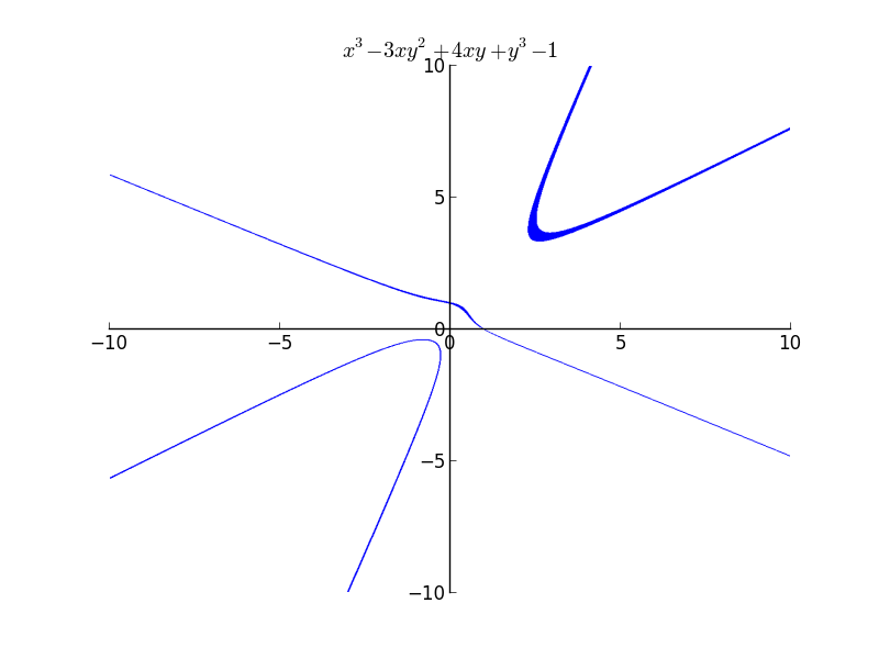
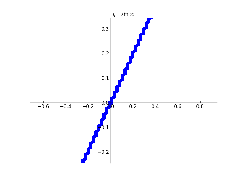
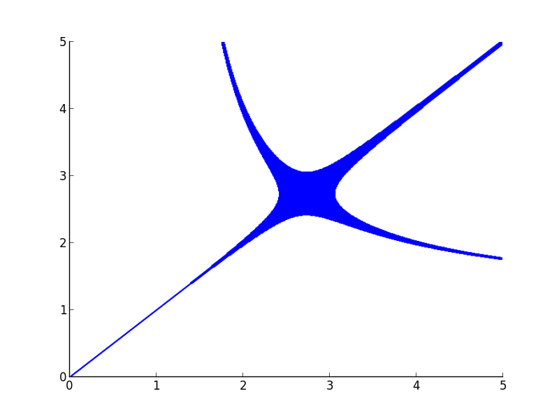
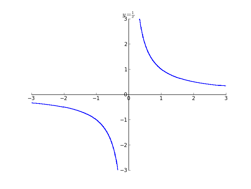
The above image illustrates a plot which does domain tracking and continuity tracking. It is not possible for interval arithmetic without tracking, to decide whether to draw the plots near zero. But with continuity tracking we get an accurate plot.

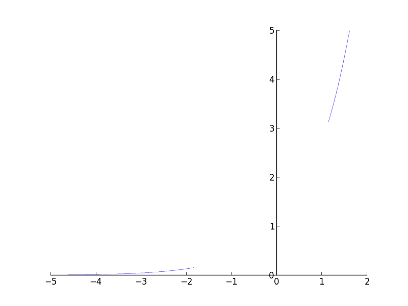
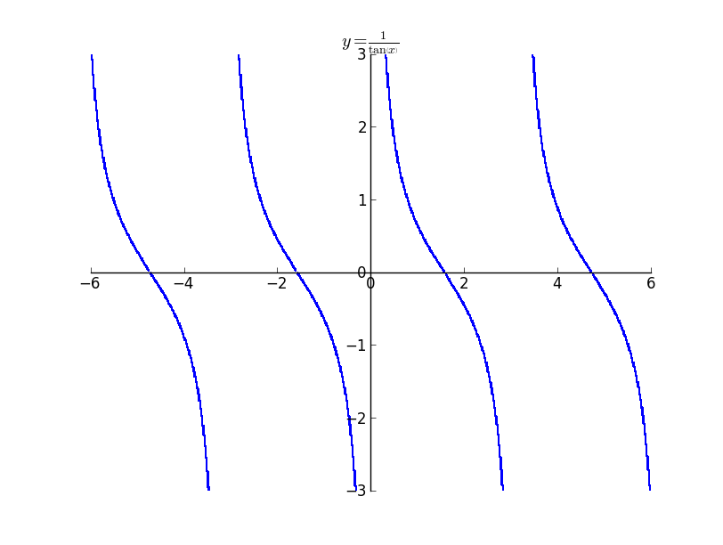
The above plot is that of $y = \frac{1}{\tan{\left (x \right )}}$ . It is possible to see the small discontinuity near multiples of $\pi / 2$ as $\pi / 2$ is not there in the domain of the expression.

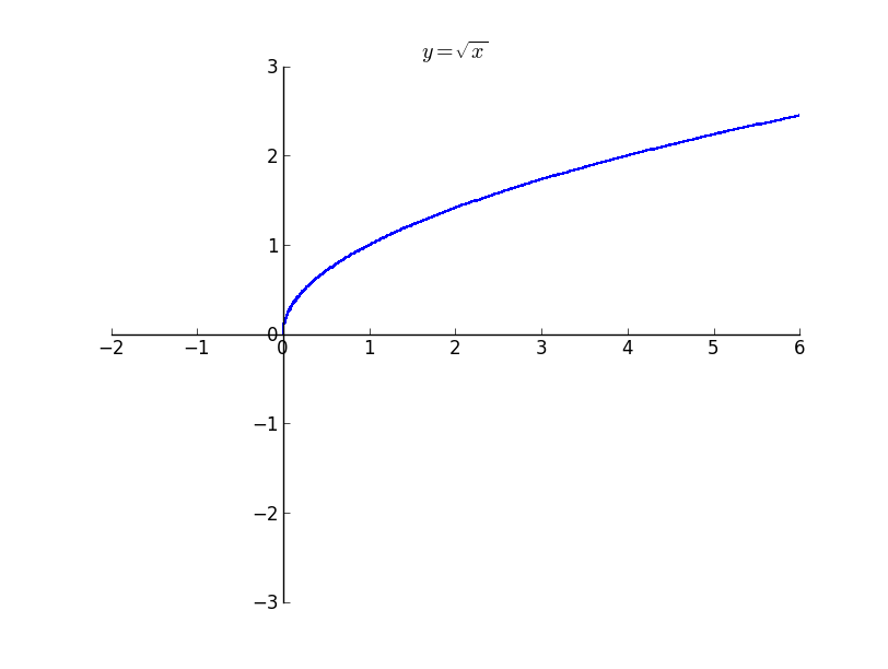
The above plot illustrates how sqrt does not plot anything outside its domain. Even though it appears not that significant, it becomes significant when the huge expression is provided as the argument to the function.

Illustrations of more plots

Plot of $y^{2}=x^{3}-x$

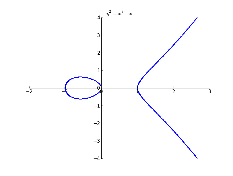
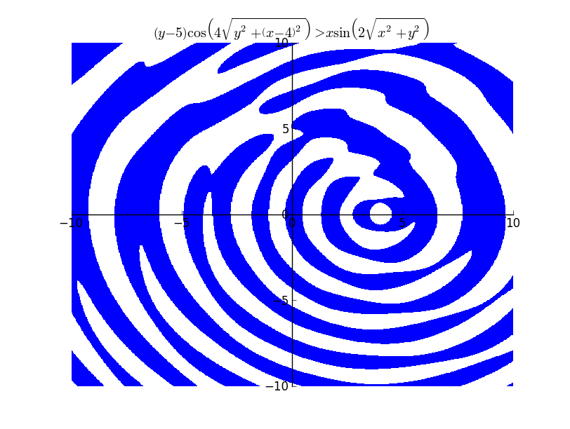
The above plot took 19.26 seconds to render.

Problems

The problem with plots using interval arithmetic is that the errors increases with the length of the expression as the it takes the lowest and the uppermost bounds. It is possible to see the effect of errors in the following plot. It is possible to see the line thickens when the expression reaches a maximum or an minimum. This is due to the error creeping in. The interval becomes wide even at the smallest of the x interval.

It is better illustrated in the plot below. It is possible to see the width of the line increasing and then decreasing.

Then next problem is that of rasterization. In order to avoid rasterization I tried using the Matplotlib’s contourf function which implements the marching squares algorithm. Though it smoothens the curves, still there is fair bit of rasterization. The plot below is a zoomed version of $y=sin(x)$

Presently the plotting function supports plotting of expressions containing cos, sin, tan, exp, log, sqrt, atan. Implementing more functions is fairly easy. I should be able to finish most of the expressions that can be implemented in the next week. I will look into implementing plotting implicit equations for expressions which cannot be implemented using interval arithmetic.